In this post we will analyze the equations for the statistical wave model presented in Tessendorf's paper[1] on simulating ocean water. In the previous post we used the discrete Fourier transform to generate our wave height field. We will proceed with the analysis in order to implement our own fast Fourier transform. With this implementation at our disposal we will be able to achieve interactive frame rates. Below are two screen captures of our result. The first uses a version of the shader from the post on lighting and environment mapping in addition to the linear fog factor discussed in the previous post. The second is a rendering of the surface geometry.

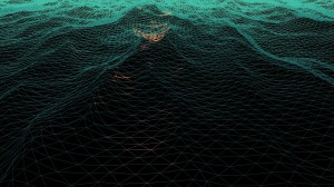
Below are the respective video captures.
We will start with the equation we arrived at in the previous post which describes the wave height at a location \((x,z)\) in terms of our indices, \(n'\) and \(m'\).
\begin{align*}
h'(x,z,t) &= \sum_{m'=0}^{M-1} \sum_{n'=0}^{N-1} \tilde{h}'(n',m',t)\exp\left(\frac{ix(2\pi n' - \pi N)}{L_x} + \frac{iz(2\pi m' - \pi M)}{L_z}\right) \\
\end{align*}
We can rearrange this equation as below,
\begin{align*}
h'(x,z,t) &= \sum_{m'=0}^{M-1} \sum_{n'=0}^{N-1} \tilde{h}'(n',m',t)\exp\left(\frac{ix(2\pi n' - \pi N)}{L_x}\right) \exp\left(\frac{iz(2\pi m' - \pi M)}{L_z}\right) \\
h'(x,z,t) &= \sum_{m'=0}^{M-1} \exp\left(\frac{iz(2\pi m' - \pi M)}{L_z}\right) \left( \sum_{n'=0}^{N-1} \tilde{h}'(n',m',t)\exp\left(\frac{ix(2\pi n' - \pi N)}{L_x}\right)\right) \\
\end{align*}
Thus, our two-dimensional discrete Fourier transform can be written as two one-dimensional discrete Fourier transforms.
\begin{align*}
h'(x,z,t) &= \sum_{m'=0}^{M-1} \exp\left(\frac{iz(2\pi m' - \pi M)}{L_z}\right) h''(x,m',t) \tag{3} \\
h''(x,m',t) &= \sum_{n'=0}^{N-1} \exp\left(\frac{ix(2\pi n' - \pi N)}{L_x}\right) \tilde{h}'(n',m',t) \tag{4} \\
\end{align*}
For now we will focus on \(h''\). The fast Fourier transform will generate a wave height field at discrete points,
\begin{align*}
(x,z) &= \left(\frac{(n'-N/2)L_x}{N},\frac{(m'-M/2)L_z}{M}\right) \\
\end{align*}
We will generate the wave height field for,
\begin{align*}
(x,z) &= (n'-N/2,m'-M/2) \\
\end{align*}
by letting \(L_x=N\) and \(L_z=M\). \(h''\) then becomes,
\begin{align*}
h''(x,m',t) &= \sum_{n'=0}^{N-1} \exp\left(\frac{ix(2\pi n' - \pi N)}{N}\right) \tilde{h}'(n',m',t)\\
&= \sum_{n'=0}^{N-1} \exp\left(\frac{i2\pi n' x}{N}\right)\exp\left(-i\pi x\right) \tilde{h}'(n',m',t) \tag{1}\\
&= -1^x\left\{\sum_{n'=0}^{N-1} \exp\left(\frac{i2\pi n' x}{N}\right) \tilde{h}'(n',m',t)\right\} \tag{2}\\
\end{align*}
We can split \(h''\) into the sum over the even indices and the sum over the odd indices as below, provided \(N\ge2\),
\begin{align*}
h''(x,m',t) =& -1^x\left\{\sum_{n'=0}^{N-1} \exp\left(\frac{i2\pi n' x}{N}\right) \tilde{h}'(n',m',t)\right\} \\
=& -1^x\left\{\sum_{n'=0}^{\frac{N}{2}-1} \exp\left(\frac{i2\pi (2n') x}{N}\right) \tilde{h}'(2n',m',t)\right\} + \\
& -1^x\left\{\sum_{n'=0}^{\frac{N}{2}-1} \exp\left(\frac{i2\pi (2n'+1) x}{N}\right) \tilde{h}'(2n'+1,m',t)\right\} \\
=& -1^x\left\{\sum_{n'=0}^{\frac{N}{2}-1} \exp\left(\frac{i2\pi n' x}{\frac{N}{2}}\right) \tilde{h}'(2n',m',t)\right\} + \\
& -1^x\left\{\sum_{n'=0}^{\frac{N}{2}-1} \exp\left(\frac{i2\pi n' x}{\frac{N}{2}}\right) \exp\left(\frac{i2\pi x}{N}\right) \tilde{h}'(2n'+1,m',t)\right\} \\
\end{align*}
Now, if we let,
\begin{align*}
T_N^x &= \exp\left(\frac{i2\pi x}{N}\right) \\
\end{align*}
We can rewrite this equation as,
\begin{align*}
h''(x,m',t) =& -1^x\left\{\sum_{n'=0}^{\frac{N}{2}-1} \exp\left(\frac{i2\pi n' x}{\frac{N}{2}}\right) \tilde{h}'(2n',m',t)\right\} + \\
& -1^x\left\{ T_N^x \sum_{n'=0}^{\frac{N}{2}-1} \exp\left(\frac{i2\pi n' x}{\frac{N}{2}}\right) \tilde{h}'(2n'+1,m',t)\right\} \\
\end{align*}
For now we will eliminate the \(-1^x\) term by defining a new function, \(h'''\). Note that when we perform the second transform we will have the term, \(-1^z\).
\begin{align*}
h'''(x,m',t) =& \sum_{n'=0}^{\frac{N}{2}-1} \exp\left(\frac{i2\pi n' x}{\frac{N}{2}}\right) \tilde{h}'(2n',m',t) + \\
& T_N^x \sum_{n'=0}^{\frac{N}{2}-1} \exp\left(\frac{i2\pi n' x}{\frac{N}{2}}\right) \tilde{h}'(2n'+1,m',t) \\
\end{align*}
An additional property to observe is the value of \(h'''\) at \(x+\frac{N}{2}\),
\begin{align*}
h'''\left(x+\frac{N}{2},m',t\right) =& \sum_{n'=0}^{\frac{N}{2}-1} \exp\left(\frac{i2\pi n' (x+\frac{N}{2})}{\frac{N}{2}}\right) \tilde{h}'(2n',m',t) + \\
& T_N^{x+\frac{N}{2}} \sum_{n'=0}^{\frac{N}{2}-1} \exp\left(\frac{i2\pi n' (x+\frac{N}{2})}{\frac{N}{2}}\right) \tilde{h}'(2n'+1,m',t) \\
\end{align*}
We have,
\begin{align*}
\exp\left(\frac{i2\pi n' (x+\frac{N}{2})}{\frac{N}{2}}\right) &= \exp\left(\frac{i2\pi n' x}{\frac{N}{2}}\right)\exp\left(\frac{i2\pi \frac{N}{2}}{\frac{N}{2}}\right) \\
&= \exp\left(\frac{i2\pi n' x}{\frac{N}{2}}\right) \\
\end{align*}
and,
\begin{align*}
T_N^{x+\frac{N}{2}} &= \exp\left(\frac{i2\pi (x+\frac{N}{2})}{N}\right) \\
&= \exp\left(\frac{i2\pi x}{N}\right) \exp\left(\frac{i2\pi\frac{N}{2}}{N}\right) \\
&= -\exp\left(\frac{i2\pi x}{N}\right) \\
&= -T_N^x
\end{align*}
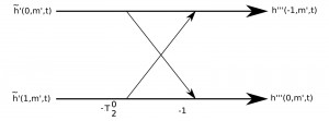
Thus, we have taken a size-\(N\) DFT and split it into two size-\(\frac{N}{2}\) DFTs where the second has been multiplied by a twiddle factor. Additionally, we have observed that the value at \(x+\frac{N}{2}\) can be obtained by reusing the intermediate computations used at \(x\).
We can generate a butterfly diagram for the case \(N=2\).
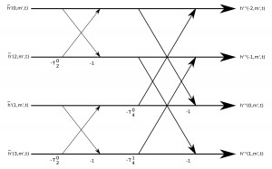
Now, provided \(N\ge4\), we can split \(h'''\) a second time.
\begin{align*}
h'''(x,m',t) =
& \sum_{n'=0}^{\frac{N}{4}-1} \exp\left(\frac{i2\pi n' x}{\frac{N}{4}}\right) \tilde{h}'(4n',m',t) + \\
& T_{\frac{N}{2}}^x \sum_{n'=0}^{\frac{N}{4}-1} \exp\left(\frac{i2\pi n' x}{\frac{N}{4}}\right) \tilde{h}'(4n'+2,m',t) + \\
& T_N^x \sum_{n'=0}^{\frac{N}{4}-1} \exp\left(\frac{i2\pi n' x}{\frac{N}{4}}\right) \tilde{h}'(4n'+1,m',t) \\
& T_N^x T_{\frac{N}{2}}^x \sum_{n'=0}^{\frac{N}{4}-1} \exp\left(\frac{i2\pi n' x}{\frac{N}{4}}\right) \tilde{h}'(4n'+3,m',t) \\
\end{align*}
Yielding the following butterfly diagram,
And the butterfly diagram for the case \(N=8\),
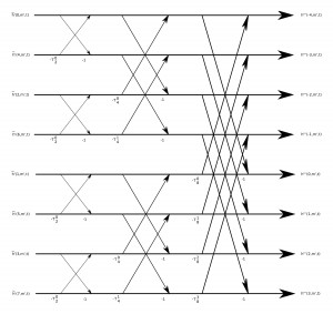
There are a few things to note. Our \(x\) values run from \(-\frac{N}{2}\) through \(\frac{N}{2}-1\), so we've used the identity, \(T_N^{x+\frac{N}{2}} = -T_N^x\), in the diagrams above. Our implementation will translate our \(x\) values by \(+\frac{N}{2}\), so we will eliminate the negative. Additionally, in our implementation we can precompute our values for \(T\). Lastly, the input values in the diagrams above are in bit-reversed order, so we will precompute an array of bit-reversed indices.
We will start with the declaration of our object to perform a fast Fourier transform. The property, c, will hold an array of intermediate values and which indicates which of the two arrays we are using. reversed will contain an array of bit-reversed indices, and T will hold the precomputed values for \(T\) in the butterfly diagram.
#ifndef FFT_H
#define FFT_H

#include <math.h>
#include "complex.h"

class cFFT {
  private:
	unsigned int N, which;
	unsigned int log_2_N;
	float pi2;
	unsigned int *reversed;
	complex **T;
	complex *c[2];
  protected:
  public:
	cFFT(unsigned int N);
	~cFFT();
	unsigned int reverse(unsigned int i);
	complex t(unsigned int x, unsigned int N);
	void fft(complex* input, complex* output, int stride, int offset);
};

#endif
Before we get to the implementation of the fast Fourier transform, we will look at the constructor. Here we simply allocate resources for our properties and precompute our bit-reversed indices in addition to our \(T\) values.
cFFT::cFFT(unsigned int N) : N(N), reversed(0), T(0), pi2(2 * M_PI) {
	c[0] = c[1] = 0;

	log_2_N = log(N)/log(2);

	reversed = new unsigned int[N];		// prep bit reversals
	for (int i = 0; i < N; i++) reversed[i] = reverse(i);

	int pow2 = 1;
	T = new complex*[log_2_N];		// prep T
	for (int i = 0; i < log_2_N; i++) {
		T[i] = new complex[pow2];
		for (int j = 0; j < pow2; j++) T[i][j] = t(j, pow2 * 2);
		pow2 *= 2;
	}

	c[0] = new complex[N];
	c[1] = new complex[N];
	which = 0;
}

cFFT::~cFFT() {
	if (c[0]) delete [] c[0];
	if (c[1]) delete [] c[1];
	if (T) {
		for (int i = 0; i < log_2_N; i++) if (T[i]) delete [] T[i];
		delete [] T;
	}
	if (reversed) delete [] reversed;
}

unsigned int cFFT::reverse(unsigned int i) {
	unsigned int res = 0;
	for (int j = 0; j < log_2_N; j++) {
		res = (res << 1) + (i & 1);
		i >>= 1;
	}
	return res;
}

complex cFFT::t(unsigned int x, unsigned int N) {
	return complex(cos(pi2 * x / N), sin(pi2 * x / N));
}
Our implementation proceeds directly from the butterfly diagrams above. From the diagrams we have \(\log_2N\) steps. In the first step we have \(\frac{N}{2}\) loops, in the second step we have \(\frac{N}{4}\) loops, and so forth. Within each loop we evaluate the intermediate values using the properties discussed above. We have added the stride and offset parameters so we can perform both transforms, one in the \(x\) direction and the other in the \(z\) direction, using the same method. This is a relatively straightforward implementation, and further optimizations could likely be made. Have a look at the FFTW library for evaluating discrete Fourier transforms.
void cFFT::fft(complex* input, complex* output, int stride, int offset) {
	for (int i = 0; i < N; i++) c[which][i] = input[reversed[i] * stride + offset];

	int loops       = N>>1;
	int size        = 1<<1;
	int size_over_2 = 1;
	int w_          = 0;
	for (int i = 1; i <= log_2_N; i++) {
		which ^= 1;
		for (int j = 0; j < loops; j++) {
			for (int k = 0; k < size_over_2; k++) {
				c[which][size * j + k] =  c[which^1][size * j + k] +
							  c[which^1][size * j + size_over_2 + k] * T[w_][k];
			}

			for (int k = size_over_2; k < size; k++) {
				c[which][size * j + k] =  c[which^1][size * j - size_over_2 + k] -
							  c[which^1][size * j + k] * T[w_][k - size_over_2];
			}
		}
		loops       >>= 1;
		size        <<= 1;
		size_over_2 <<= 1;
		w_++;
	}

	for (int i = 0; i < N; i++) output[i * stride + offset] = c[which][i];
}
Our cOcean object is similar to the one in the last post, but we have added the evaluateWavesFFT method to utilized the cFFT object. Recall the \(-1^x\) and \(-1^z\) factors above. They come into play after we perform the fast Fourier transform. Additionally, we have utilized the cFFT object to evaluate our displacements and normal vectors.
void cOcean::evaluateWavesFFT(float t) {
	float kx, kz, len, lambda = -1.0f;
	int index, index1;

	for (int m_prime = 0; m_prime < N; m_prime++) {
		kz = M_PI * (2.0f * m_prime - N) / length;
		for (int n_prime = 0; n_prime < N; n_prime++) {
			kx = M_PI*(2 * n_prime - N) / length;
			len = sqrt(kx * kx + kz * kz);
			index = m_prime * N + n_prime;

			h_tilde[index] = hTilde(t, n_prime, m_prime);
			h_tilde_slopex[index] = h_tilde[index] * complex(0, kx);
			h_tilde_slopez[index] = h_tilde[index] * complex(0, kz);
			if (len < 0.000001f) {
				h_tilde_dx[index]     = complex(0.0f, 0.0f);
				h_tilde_dz[index]     = complex(0.0f, 0.0f);
			} else {
				h_tilde_dx[index]     = h_tilde[index] * complex(0, -kx/len);
				h_tilde_dz[index]     = h_tilde[index] * complex(0, -kz/len);
			}
		}
	}

	for (int m_prime = 0; m_prime < N; m_prime++) {
		fft->fft(h_tilde, h_tilde, 1, m_prime * N);
		fft->fft(h_tilde_slopex, h_tilde_slopex, 1, m_prime * N);
		fft->fft(h_tilde_slopez, h_tilde_slopez, 1, m_prime * N);
		fft->fft(h_tilde_dx, h_tilde_dx, 1, m_prime * N);
		fft->fft(h_tilde_dz, h_tilde_dz, 1, m_prime * N);
	}
	for (int n_prime = 0; n_prime < N; n_prime++) {
		fft->fft(h_tilde, h_tilde, N, n_prime);
		fft->fft(h_tilde_slopex, h_tilde_slopex, N, n_prime);
		fft->fft(h_tilde_slopez, h_tilde_slopez, N, n_prime);
		fft->fft(h_tilde_dx, h_tilde_dx, N, n_prime);
		fft->fft(h_tilde_dz, h_tilde_dz, N, n_prime);
	}

	int sign;
	float signs[] = { 1.0f, -1.0f };
	vector3 n;
	for (int m_prime = 0; m_prime < N; m_prime++) {
		for (int n_prime = 0; n_prime < N; n_prime++) {
			index  = m_prime * N + n_prime;		// index into h_tilde..
			index1 = m_prime * Nplus1 + n_prime;	// index into vertices

			sign = signs[(n_prime + m_prime) & 1];

			h_tilde[index]     = h_tilde[index] * sign;

			// height
			vertices[index1].y = h_tilde[index].a;

			// displacement
			h_tilde_dx[index] = h_tilde_dx[index] * sign;
			h_tilde_dz[index] = h_tilde_dz[index] * sign;
			vertices[index1].x = vertices[index1].ox + h_tilde_dx[index].a * lambda;
			vertices[index1].z = vertices[index1].oz + h_tilde_dz[index].a * lambda;

			// normal
			h_tilde_slopex[index] = h_tilde_slopex[index] * sign;
			h_tilde_slopez[index] = h_tilde_slopez[index] * sign;
			n = vector3(0.0f - h_tilde_slopex[index].a, 1.0f, 0.0f - h_tilde_slopez[index].a).unit();
			vertices[index1].nx =  n.x;
			vertices[index1].ny =  n.y;
			vertices[index1].nz =  n.z;

			// for tiling
			if (n_prime == 0 && m_prime == 0) {
				vertices[index1 + N + Nplus1 * N].y = h_tilde[index].a;

				vertices[index1 + N + Nplus1 * N].x = vertices[index1 + N + Nplus1 * N].ox + h_tilde_dx[index].a * lambda;
				vertices[index1 + N + Nplus1 * N].z = vertices[index1 + N + Nplus1 * N].oz + h_tilde_dz[index].a * lambda;

				vertices[index1 + N + Nplus1 * N].nx =  n.x;
				vertices[index1 + N + Nplus1 * N].ny =  n.y;
				vertices[index1 + N + Nplus1 * N].nz =  n.z;
			}
			if (n_prime == 0) {
				vertices[index1 + N].y = h_tilde[index].a;

				vertices[index1 + N].x = vertices[index1 + N].ox + h_tilde_dx[index].a * lambda;
				vertices[index1 + N].z = vertices[index1 + N].oz + h_tilde_dz[index].a * lambda;

				vertices[index1 + N].nx =  n.x;
				vertices[index1 + N].ny =  n.y;
				vertices[index1 + N].nz =  n.z;
			}
			if (m_prime == 0) {
				vertices[index1 + Nplus1 * N].y = h_tilde[index].a;

				vertices[index1 + Nplus1 * N].x = vertices[index1 + Nplus1 * N].ox + h_tilde_dx[index].a * lambda;
				vertices[index1 + Nplus1 * N].z = vertices[index1 + Nplus1 * N].oz + h_tilde_dz[index].a * lambda;

				vertices[index1 + Nplus1 * N].nx =  n.x;
				vertices[index1 + Nplus1 * N].ny =  n.y;
				vertices[index1 + Nplus1 * N].nz =  n.z;
			}
		}
	}
}
At this point we have implemented a basic ocean simulation using a fast Fourier transform. We could proceed by optimizing our transform and utilizing the GPU in addition to adding more advanced rendering algorithms to simulate the interaction of light.
If you have any thoughts, let me know, but for now download the project and try it out.
Download this proejct: waves.fft_correction20121002.tar.bz2
References:
1. Tessendorf, Jerry. Simulating Ocean Water. In SIGGRAPH 2002 Course Notes #9 (Simulating Nature: Realistic and Interactive Techniques), ACM Press.


Comments
Thanks for your post! I wouldn't have figured how to generate the normal and choppiness vectors on my own!! (I did read J.Tessendorf's paper dozens of times but it wasn't very clear to me how to obtain those).
Author
Hey Tom..
Glad I could help. Some of those details are a bit tricky. It took me a while to work through them myself.
Care to explain the sign flipping thing? I've discovered I had to do the same thing in my ocean renderer, when using both FFTW and cuFFT. But I've never seen any explanation of why you have to do it...
Author
Hey Anders..
I was curious about that when I saw it myself. I've labeled the equations in the post, \((1)\) and \((2)\), where we extract the \((-1)^x\) factor from the summation.
We used Euler's formula,
\begin{align*}
\exp(ix) &= \cos x + i\sin x \\
\end{align*}
and applied it to our factor,
\begin{align*}
\exp\left(-i\pi x\right) &= \left(\exp\left(-i\pi\right)\right)^x \\
&= \left(\cos \left(-\pi\right) + i\sin\left(-\pi\right)\right)^x \\
&= \left(\cos \left(-\pi\right)\right)^x \\
&= \left(-1\right)^x \\
\end{align*}
Of course you have a similar term for the second transform, \((-1)^z\), so you end up with, \((-1)^{x+z}\).
I hope that answers your question.
Thanks for your answer, however it doesn't really answer what I was wondering. Maybe my question was poorly formulated...
Anyways, what I want to know is, WHY do we have to do this sign flipping? Is it something we would also get with a regular inverse Fourier transform, or is it something special to FFTs? Or is it something special for this (and other similar) problem domain, i.e. for some problems you need to flip the sign and for some you don't?
Your blog is the first among MANY sites I've visited that even mention it, so for a while, I was under the impression I had done something wrong in my algorithm (even though with the sign flipping, the water looked really nice).
Author
The discrete Fourier transform is a summation over the indices, \(0, 1, ... N-1\). The wave height field for this particular problem is defined on the grid running from \(-N/2, -N/2+1, ... N/2-1\). In order to apply a discrete/fast Fourier transform the grid for this specific problem needs to be translated. The sign flipping is a consequence of translating the grid by \(+N/2\). The term, \((-1)^x\), is not a part of the transform, which is why it is applied after the transform is performed.
Actually, I ran into a similar situation in my post on generating terrain. This also involved translating the grid by \(+N/2\) so the indices run from \(0, 1, ... N-1\). I had to perform the sign flipping in this case as well.
It is not a property of the transform. Some problems have the grid defined in such a way that a translation is required in order to perform the transform.
Hope that helps.
Thanks for the awesome post. I've read tessendorfs work several months ago and thought: That's what I need but, damn, this gonna be tricky.
With your post I was able to adopt it in java (using jme3 and jtransform) and it works like a charm.
Author
Hey.. that's cool you were able to adapt it. Thanks for the comment!
btw. I can't find the choppy-part in the code. Can you show it because it seems I have problems to use it.
Author
It's been a while, but in the evaluateWavesFFT method the h_tilde_dx and h_tilde_dz arrays hold the displacement. These are evaluated using the transform. In the final loop of that method the displacement is then applied to the vertices with this code (lines 58 and 59 above):
vertices[index1].x = vertices[index1].ox + h_tilde_dx[index].a * lambda;

vertices[index1].z = vertices[index1].oz + h_tilde_dz[index].a * lambda;
If you change this code to:
vertices[index1].x = vertices[index1].ox;

vertices[index1].z = vertices[index1].oz;
you should be good, minus the chopiness.
I think this post has a few more details in regard to evaluating the displacement vector. That process should be the same here, except here we exploit the fast Fourier transform.
Let me know if that doesn't clarify anything, and I'll have a closer look at it.
Ah thank you. Also I found a bug in my Complex-object. Now it looks like expected.
thanks.
If anybody is interested in the Java-Version. The code is opensource and uploaded on sourceforge: http://sourceforge.net/projects/oceanmonkey/
It's still a prototype but the proof of concept does its job.
Hi
Can you explain a little bit more about the use of "Stride" and "offset" variable ?
I have some difficulty visualizing its use
Author
Hey Juan..
To use an example, in the
cOcean::evaluateWavesFFT()method we call thecFFT::fft()method on theh_tildearray. Theh_tildearray is a one-dimensional array storing, I think, \(N \times N\) values, so we are representing our two-dimensions with an array of only one-dimension. The first time we call thefft()method, we use a stride of 1 and an offset ofm_prime * N. In this casem_prime * Nrepresents the row and a stride of 1 allows us to pull neighboring values along that row. The secondfft()call uses a stride ofNand an offset ofn_prime. In this casen_primerepresents the column and a stride ofNallows us to use those values along that column.Basically, the stride and offset allow us to handle a one-dimensional array as though it were two-dimensional. Is that clear? Let me know if it is not, and I'll try to come up with a clearer explanation.
That explains it.
But what happened to h´(x,z,t) (after you split it into a sum of 2 one dimensional DFTs) ?
From what i can see the math only cover the second factor h´´(x,z,t)
Author
Your right. We only mess with the \(h''\) term.
I've labeled the equations above, 3 and 4, where you refer to the split. Here we have two one-dimensional Fourier transforms. In the
cOcean::evaluateWavesFFT()method we first populateh_tildewith our \(\tilde{h}'\) values for equation 4. The first Fourier transform, equation 4, is handled first in thecOcean::evaluateWavesFFT()method (along the rows using a stride of 1). The second transform, equation 3, is applied immediately after that (along the columns using a stride ofN).We still have the \(-1^x\) and \(-1^z\) terms that need to be applied, but we were able to pull these completely out of the summations, so these terms were applied last, after both transforms. I think maybe the key is to seeing that \(h'\) from equation 3 is just another Fourier transform once we extract the \(-1^z\) term.
This is a fantastic explanation, especially as you include source code too!
I've ported it to Java for Android and made some simple optimisations and it runs fine, though sadly my phone is too slow to really handle anything above a 32x32 grid, which does somewhat reduce the effect!
Author
Cool! Do you have any screen captures?
OK, I knocked up a more general app you can download at https://play.google.com/store/apps/details?id=uk.co.jackhollow.android.oceanfft.
Even if you're an apple boy, you can see the screenshots at least!
The FFT evaluation is still pretty slow compared to the C++ version, and is the bottleneck in the whole app. I don't how to optimise it any more though; fundamentally it's doing a lot of iteration loops.
bevis
I am wondering why lambda is -1 in your code. Is it caused by the "translation" of the frequency spectrum to the 0...N domain?
float lambda = -1.0f;

vertices[index1].x = vertices[index1].ox + h_tilde_dx[index].a * lambda;

vertices[index1].z = vertices[index1].oz + h_tilde_dz[index].a * lambda;
Author
It isn't due to the translation; that should be handled by the
signvariable. I don't recall if I had a good reason for using \(-1\) other than it looked visually appealing. When \(\lambda = -1\), the peaks are sharpened and the troughs are broadened. If \(\lambda\) where positive, the opposite would be true: the peaks would become broad and the troughs would become narrow, which didn't appear to be visually accurate.Thanks. You are right, same for me, I need λ equal -1 to broaden the "valleys".
Right now I am meddling with another issue: the scaling of the heights is not right e.g. I get heights with a minimum value of -13 and maximum value of +14 for a spectrum generated with size parameter 40. If I rescale x and z by factor 10 it looks ok. Did you encounter a similar issue?
Author
Hey icicle.. another question made me realize I missed a \(-1\) when I evaluated
Din theh_D_and_n()method. I think that was ultimately why I needed \(\lambda\) to be negative.. to correct this mistake.Now I am confused 🙂 I am rather confident I implemented it correctly, seems like I screwed a sign somewhere up, too, but I cannot find it.
At least I figured out how to keep xz / y scale sane without fiddling around with magic constants.
AFAICT your implementation of the displacement computation in h_D_and_n is correct, I did it the same way without having looked at your code. Where exactly is a -1 missing, because it seems I made the same mistake, and you could point me in the right direction 🙂
Author
Hey icicle..
I'm having trouble locating the missing -1. I'm not so sure it's missing any more :).
Hey. I checked with MATLAB using complex numbers explicitely. It seems we did not miss a -1.
Amazing!
I move your code in DX,everything ok but the ocean shape just freezy with some little shaking. Have you encountered similar problems?
Thanks in advance!
Nice work. Do you mind if I port this to Unity and put it up on my blog?
I will link your blog as the original source of course and provide a download of the Unity project files.
Author
Hey Scrawk..
I don't mind. Keep me posted. I'd be interested in checking it out.
Thanks.
http://scrawkblog.com/2013/08/04/ocean-waves-using-phillips-spectrum-in-unity/
Pingback: Ocean waves using phillips Spectrum in Unity | scrawkblog
hey why do you do the bit reversal? I don't recall seeing that in the Tessendorfs paper
Author
Hey Connor..
The bit reversal is not specifically related to Tessendorf's paper. The bit reversal is part of the derivation of the algorithm for the Fast Fourier Transform. These links might help shed some light..
http://en.wikipedia.org/wiki/Bit-reversal_permutation
http://www.dspguide.com/ch12/2.htm
How do I compile and run this project on ubuntu..?
It says Error 1 SDL/SDL.h is missing
Hey Keith,
first of all a big thanks for your tutorial on water sim, this has helped me a lot to understand the parameter setup.
I have a question concerning the FFT functions. Im trying to use kiss_fft instead of your functions, do you have any hints on how to change the code, I have used the kiss_fft functions like this
for (int m_prime = 0; m_prime < N; m_prime++) {
kiss_fft(fft, &h_tilde[m_prime * N], &h_tilde[m_prime * N]);
kiss_fft(fft, &h_tilde_slopex[m_prime * N], &h_tilde_slopex[m_prime * N]);
kiss_fft(fft, &h_tilde_slopez[m_prime * N], &h_tilde_slopez[m_prime * N]);
kiss_fft(fft, &h_tilde_dx[m_prime * N], &h_tilde_dx[m_prime * N]);
kiss_fft(fft, &h_tilde_dz[m_prime * N], &h_tilde_dz[m_prime * N]);
}
for (int n_prime = 0; n_prime < N; n_prime++) {
kiss_fft_stride(fft, &h_tilde[n_prime], &h_tilde[n_prime], N);
kiss_fft_stride(fft, &h_tilde_slopex[n_prime], &h_tilde_slopex[n_prime], N);
kiss_fft_stride(fft, &h_tilde_slopez[n_prime], &h_tilde_slopez[n_prime], N);
kiss_fft_stride(fft, &h_tilde_dx[n_prime], &h_tilde_dx[n_prime], N);
kiss_fft_stride(fft, &h_tilde_dz[n_prime], &h_tilde_dz[n_prime], N);
}
so the offset is done beforehand(by getting the pointer &h_tilde[n_prime] or &h_tilde[m_prime * N] as the kiss functions do not provide an offset.
But this does not seem to work correctly. I have checked that the kiss lib also uses Cooley Tukey FFT, so I am not sure what exactly the problem is, as I am not very firm with FFT Algorithms.
Hope you can help me with that, feel free to contact me by my mail,
Best Regards!!!
Drato
Pingback: Compute Shader FFT of size 32 |
Hey! Great article! I want to use this technique in my OpenGL engine which is a *crossplatform* thingy. I hope this will run smooth after some optimizations.
Have anybody tried to port it to iOS/WP/Android.. whatever?!
Thanks!
I'm just trying to build a high level understanding of Tessendorf's paper and came across this. My experience with FFT's is limited to acoustics. I've used an FFT to convert a chunk of power-vs-time data to frequency-vs-amplitude data and an inverse FFT to convert back.
In this case, it seems we are converting between height-vs-position and frequency-vs-amplitude-vs-phase and all of this changes over time. Can you help me understand what are actually the two domains that we are converting between here? If I could form an analogy in my mind between this and acoustics, I think it will all click for me.
Nevermind, I think I got it. Acoustic time is analogous to position here. Acoustic frequency Hz is analogous to frequency as peaks/distance. And the phases are used to animate the spectrum over time.
Awesome work. Thank you very much 🙂
I'm currently trying to add foam simulation using the Jacobian from the paper.
I approximate the partial derivative using small offsets on the grid but its look weird.
float dx = vertices[index1].x - vertices[index].x;
float dy = vertices[index1].z - vertices[index].z;
float dxx = (h_tilde_dx[index1].a - h_tilde_dx[index].a) / dx;
float dyy = (h_tilde_dz[index1].a - h_tilde_dz[index].a) / dy;
float dyx = (h_tilde_dz[index1].a - h_tilde_dz[index].a) / dx;
float jxx = 1.0f + lambda * dxx;
float jyy = 1.0f + lambda * dyy;
float jyx = lambda * dyx;
float jxy = jyx;
vertices[index].jacobian = jxx * jyy - jxy * jyx;
Does anybody knows how to properly calculate it ?
where did you apply the (-1)^x and (-1)^z? and why did you remove these terms in h
′′′?
Aren't you suppose to invert the result it by multiplying by: 1/(N*N)
I only see you multiply by a sign and nothing else?
I think I spotted a mistake in the butterfly diagram with the negative N/2 interval. In fact, I tried to understand the algorithm by looking at it, and just couldn't work it out. So I tried to do the same by shifting by N/2 like you suggested, and the math simply worked. So I looked a bit into why the graph was giving wrong results.
The problem is with the sign of the T factors. Consider the case with N=4. The T factors with N=4 are properly signed. However, the ones with N=2 are not. For example, when calculating h'''[-2], the factors h'[2] is multiplied by -T02. This is incorrect, it should be +T02. The reason is that x=-2 is actually x=0-N, not N/2. So the sign flips twice, and the factor has to be positive.
Just wanted to point this out. The algorithm works fine because the shift by N/2 solves all issues with signs.
Wait, is this an FFT or an IFFT ? Your twiddles have positive values in the exponential rather than negatives, leads me to think you are using IFFT since the definition for it is exp(i2pi) rather than exp(-i2pi) but you don't invert by dividing through by N at the end so you're not inverting - but isn't Phillips spectrum in the frequency domain so you are meant to invert...?